1 Introduction
This note addresses the extent to which telescope tracking imperfections contribute to image degradation. We consider telescope tracking to be distinct from oscillations in either the optical support elements or axis control systems. Any uncorrected residuals from periodic drive system errors or from encoder errors contribute to the tracking image quality budget term. In addition, if the pointing model departs from the actual motion of the sky, the resulting boresight tracking errors also contribute to the tracking term. We therefore define tracking errors as image motion with Fourier components below 0.1 Hz. The long exposures used here (10–30 sec) have limited sensitivity to frequencies above 0.1 Hz.
The RMS residuals when the telescope conducts pointing tests across the sky bear upon absolute astrometric performance. Imagine a map of the magnitude of the boresight pointing error across azimuth and elevation. The gradient in this map, integrated over the duration of an exposure, is one way to think about the tracking contribution to image blur.
The pointing model and its associated lookup tables directly impact the tracking performance of the system. It is therefore important to clearly register the pointing model in place when tracking blur is measured.
For a single stellar PSF, the uncertainty in the determination of its centroid in x and y is given by \(\sigma=\) FWHM/SNR, where FWHM is the Full Width at Half Maximum for the PSF and SNR is the signal to noise ratio for that stellar image. For the tests described here the objects are all substantially brighter than the sky background and the SNR is effectively the square root of the number of photons collected from the source. The typical objects used below have total fluxes of over 100,000 ADU, so that the uncertainty in their centroids (even in bad seeing of 2 arcsec that we had for this run) should be established to a measurement uncertainty of (2 arcsec/sqrt(1E5)) \(\sim\) a few milliarcsec. The jitter in centroid positions we see below are therefore unlikely to arise from measurement uncertainties.
2 Axis Rates vs. Altitude, Azimuth, and Declination
For an Alt-Az telescope that is tracking the sky, the three axes (azimuth, rotator, and elevation) run at rates that depend on azimuth, elevation, and distance from the pole. The most stressing case for the elevation axis is when the telescope points E or W, but that maximum rate is close to the sidereal rate of 15 arcsec/sec.
The most stressing case for the azimuth axis and the rotator is as the telescope approaches the zenith. When tracking an object across the meridian. When the telescope points straight up while tracking the azimuth rate is formally infinite- since the telescope and dome have to whip around from pointing E to pointing W.
At the South Celestial Pole (SCP) the elevation and azimuth rates are zero, and the rotator spins at 15 arcsec/sec. This makes the SCP a good location for a control data set when the elevation and azimuth rates are essentially zero.
Our zone of avoidance at the zenith for Aux Tel is set by the maximum rate of the rotator, to be an elevation of 86.5 deg (check this).
3 Data Collection on Nov 3–4 and Nov 4–5 2021
- Need:
- passbands
- coord ranges
- exp times (check them)
| Target | \(t_{exp}\) | Azimuth | Elevation | Day Obs | Seq Nums | Notes |
|---|---|---|---|---|---|---|
| TIC 181887100 | 30 | Az1 | El 1 | 20211103 | 289 – 349 | RR Ly |
| HD 16591 | 30 | 151–zz | 76–bb | 20211103 | 350 – 391 | Bright! Main target saturated |
| HD 16591 | 30 | 392 | Earthquake image, omit | |||
| HD 16591 | 30 | az range | elev range | 20211103 | 393 – 437 | dome obscured |
| TIC 181887100 | 30 | Az1 | El 1 | 20211103 | 622 – 682 | RR Ly |
| TIC 181887100 | 30 | Az1 | El 1 | 20211103 | 622 – 682 | 645, 656, 665, 672 show jumps in the images |
| TIC 181887100 | 30 | Az1 | El 1 | 20211104 | 189 – 248 | RR Ly |
| TYC 9502-41-1 | 15 | 180 | 30 | 20211104 | 614 – 853 | SCP control data set |
| HD 94128 | 30 | Az1 | El 1 | 20211104 | 855 – 927 | elevation axis test |
| TIC 181887100 | 30 | Az1 | El 1 | 20211104 | 963 – 1002 | RR Ly |
4 Analysis
4.1 South Celestial Pole- Control Data Set
The images taken over the course of an hour on 20211104 when the telescope was pointed at the South Celestial Pole constitute a control data set that can help distinguish factors like drift in the mirror support systems from axis control errors. Figure 1 and Figure 2 show the x and y motion, in arcsec, over the 1.17 hour sequence. There is a monotonic drift in both the x and y axes of 2 arcsec over this duration, as well as short-term variability that substantially exceeds the position uncertainty estimate of a few milliarcsec = FWHM/SNR. These reductions were performed on the star at x,y =2756, 2416, designated as object 21 in the SCP image shown in Figure 3.
The centroid of this object was measured on a subset of the frames using the astropy tool DAOstarfinder, within the Jupiter notebook
PSFexam3.ipynb. The version of this that we used is included in the GitHub repository for this technical note.
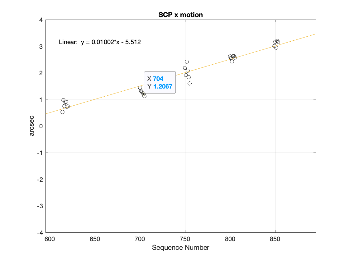
Figure 1 X direction motion at SCP for a 1.17 hour sequence.
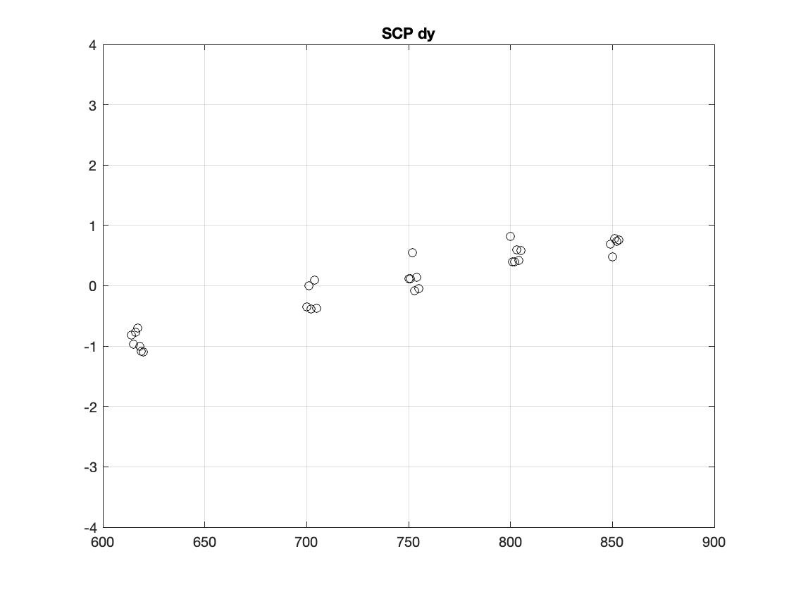
Figure 2 Y direction motion at SCP for a 1.17 hour sequence.
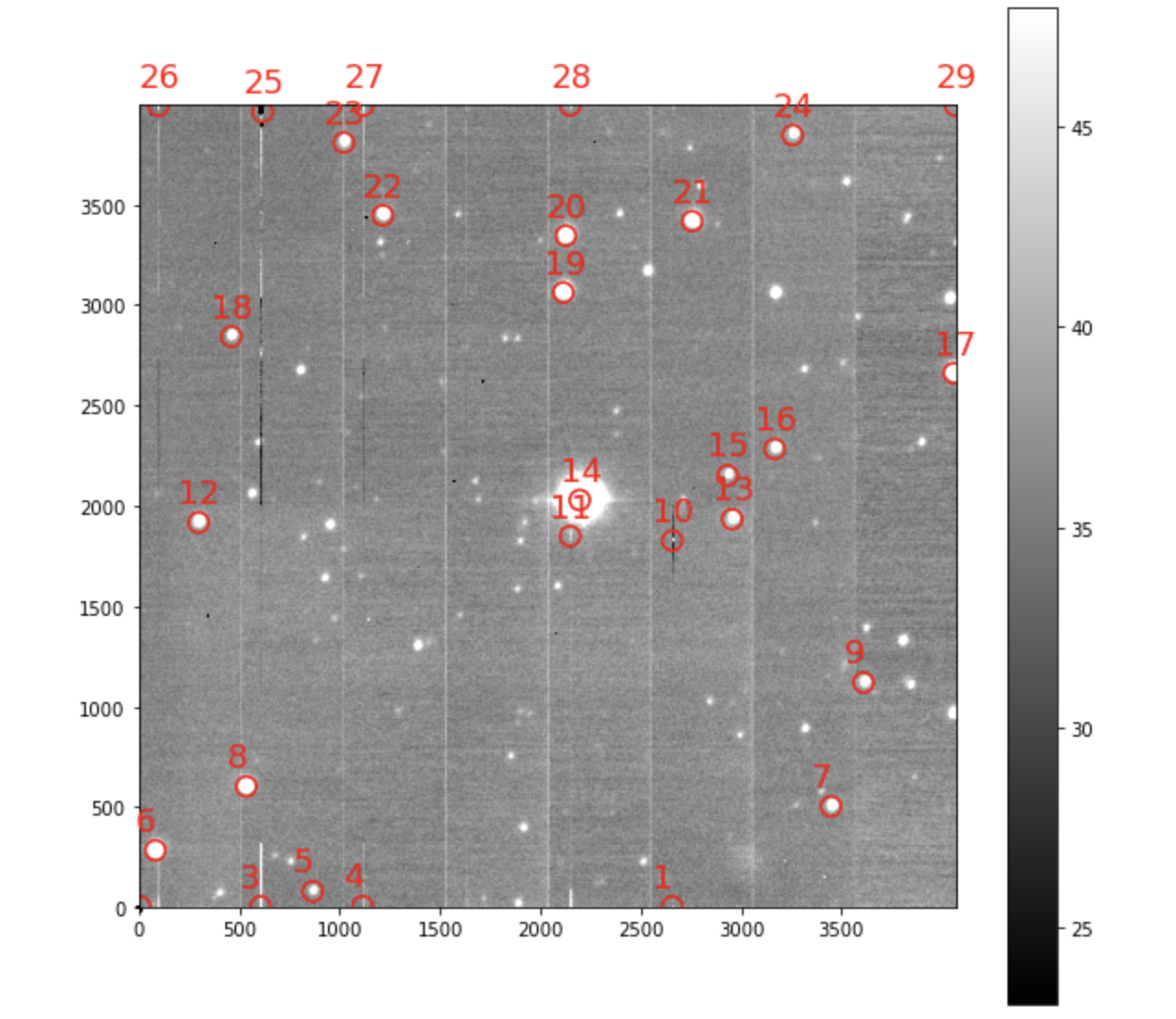
Figure 3 The single star used for the motion analysis is designated as object 21 in this image.
We tentatively conclude from the SCP test that there is a limit to boresight stability of order \(\sqrt{2}\) * 2 arcsec over 1.17 hours, or roughly 0.5 milliarcsec per second of exposure time even with the telescope essentially stationary. In a nominal 15 second exposure this term would contribute around 7 mas * (\(t_{exp}\) /15 sec) of image blur.
In addition there is a higher-frequency that manifests in the motion in x and y between adjacent images. The standard deviation of the residuals for a straight-line fit is \(\sigma=\) 0.18 arcsec. This origin of this scatter is presently unclear, and it certainly dominates the centroid motion on short time scales.
4.2 Elevation Axis Tests
4.3 Azimuth and Rotation Axis Tests
The image sequence taken 20211103, seq numbers 350 – 360 gives us an indication of the image motion as the telescope tracks up towards the zenith. The centroid of the star at (3252,3113) was used to determine image motion. Figure 4 and Figure 5 show the star’s displacement over the 345 seconds spanned by those images. The displacements in x and y are not strictly linear in time, and span 1.7 and 1.6 arcsec, respectively.
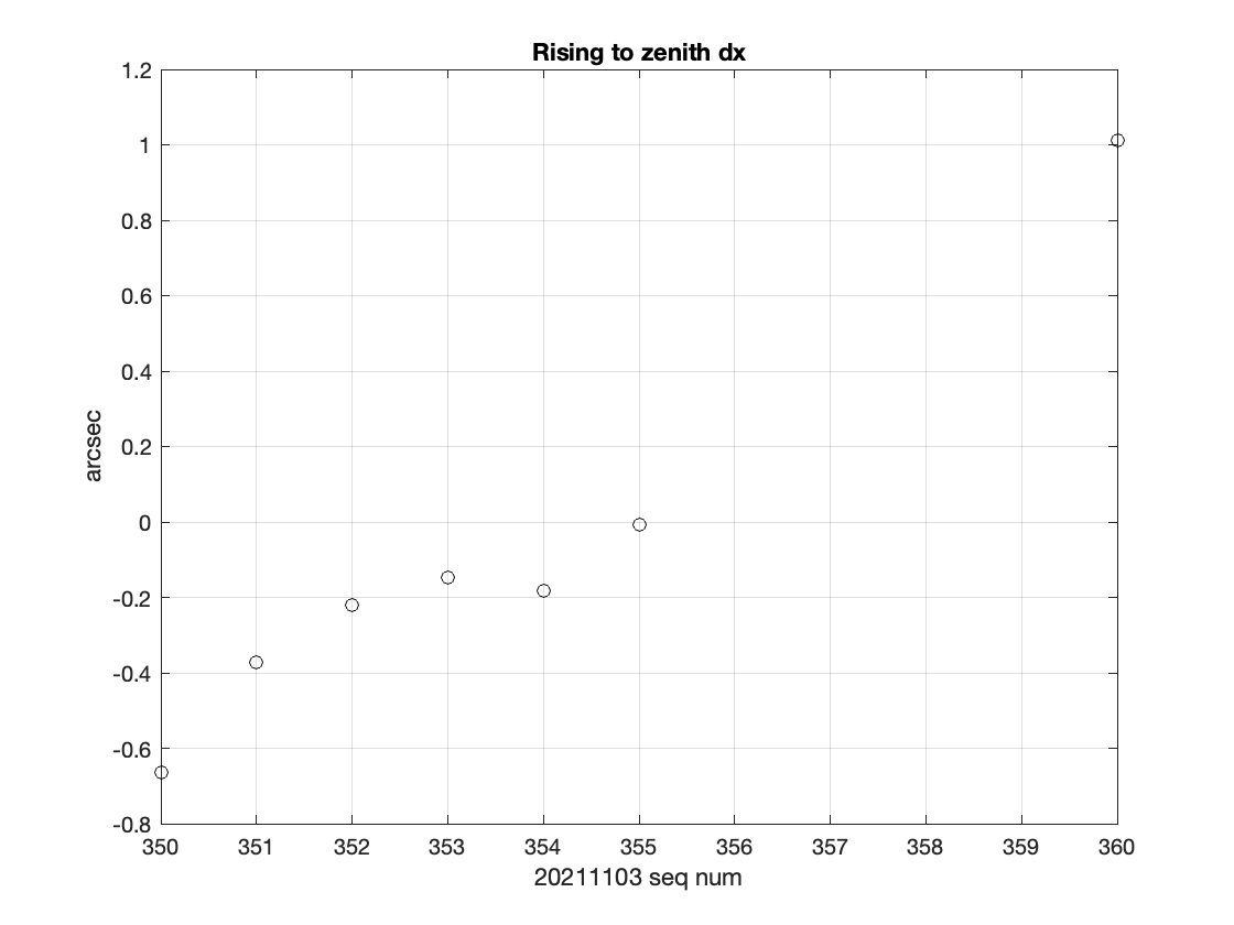
Figure 4 X direction motion tracking towards the zenith at an elevation at Az=155 Elevation = 77 for a 345 second long image sequence.
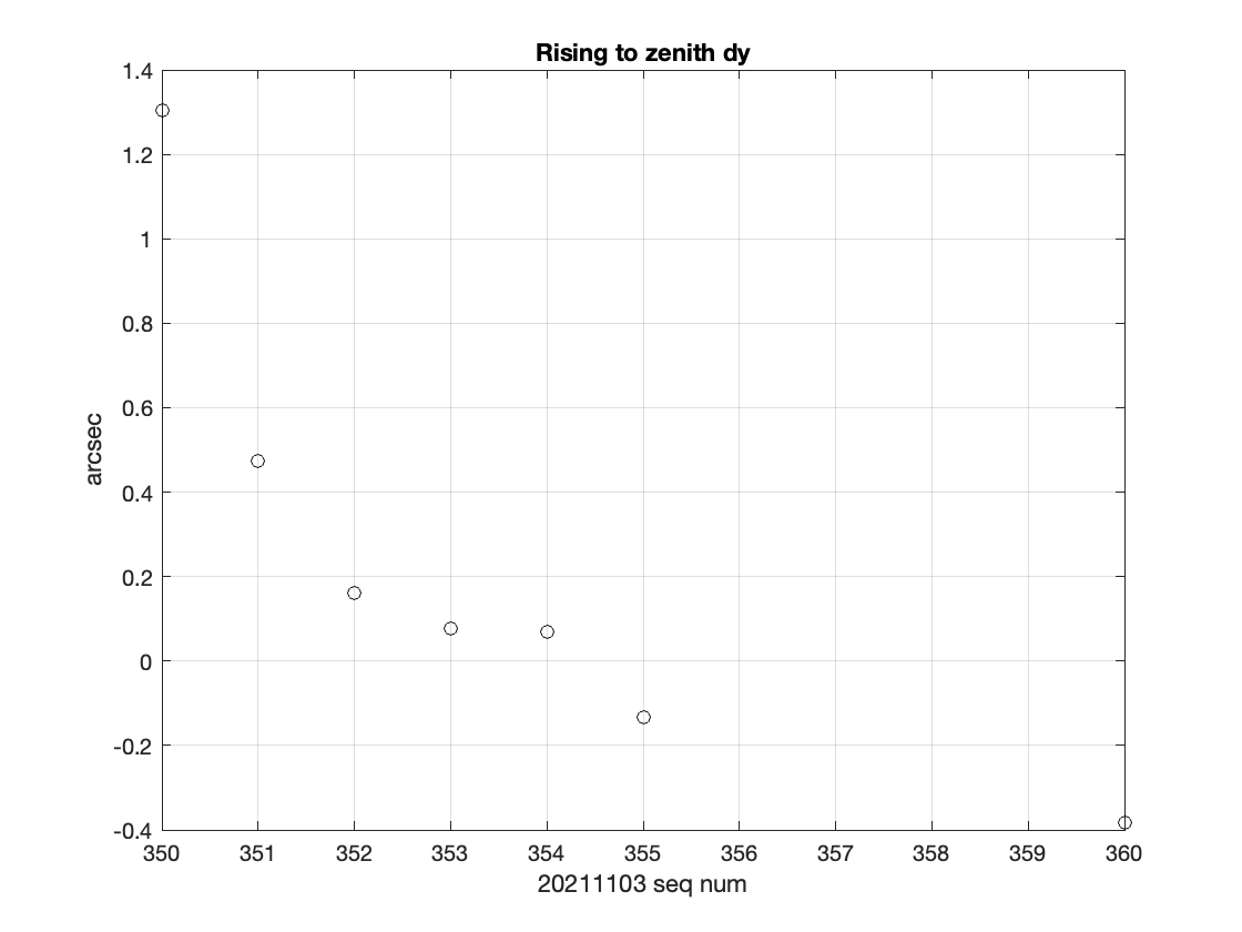
Figure 5 Y direction motion tracking towards the zenith at an elevation at Az=155 Elevation = 77 for a 345 second long image sequence.
This tracking error would induce an image blur of (again accounting for the magnitude of the displacement in the two directions) \(\sqrt{2}\) *1.6*(\(t_{exp}/345)\sim\) 0.1 arcsec in a nominal 15 second exposure.
5 Conclusions
This overall approach seems sound. The clear difference between performance at the SCP and when tracking towards the zenith.
There appears to be a steady drift in the boresight when pointing towards the S pole, with the telescope stationary. If we assume the drive system is actively servoing the elevation and azimuth axes to their correct (and essentially static) positions, this presumably arises from motion of one or both of the mirror support systems. Over the course of an hour this drift accumulates to an offset of about 2 arcseconds.
There are multiple frames with apparent bistability in pointing, at az=XX and elevation = YY (need to look up pointing for frames 645-672 on 20211103). These happened while tracking the sky, and are not an instance of the shutter opening before a slew was finished.
6 Image Quality Terms from Telescope Tracking
After attempting to isolate the contributions to the current Aux Tel image quality budget from telescope tracking we arrive at an initial allocation shown in Table 2. This assumes that a displacement of \(\theta\) in the boresight introduces a term in the FWHM that is equal to \(\theta\). That oversimplification needs to be refined.
For context, the allocation in the image quality budget to tracking errors for the 8.4m Simonyi Telescope is 0.07 arcsec, presumably for the baseline 15 sec LSST exposure time. The performance of the Aux Tel is already close to this specification, pending a more sophisticated conversion from image displacement to FWHM contribution. Longer exposures will suffer an proportional increase in cumulative tracking errors.
| Conditions | Image FWHM estimate for 15 sec exposure |
|---|---|
|
0.007 arcsec |
| Tracking towards zenith, 78 deg elevation | 0.1 arcsec |
7 Recommendations for Further Work
- Develop an automated tracking diagnostic capability, as outlined in the subsection below, then re-analyze the full data set obtained during this run.
- Obtain uninterrupted track across meridian, avoiding earthquakes this time!
- Obtain tracking performance data as a function of hour angle and declination, in half-hour long intervals using successive 15 second exposures.
- Measure centroid motion RMS vs. exposure time, at SCP, for further image quality diagnostics.
- Measure correlations of displacements using multiple stars, to see if the adjacent-frame jitter is common mode or not.
- Perform full time series analysis, and analysis vs azimuth and elevation, to look for periodic errors
- Attempt guider-mode operation of Aux Tel.
- Add pointing model to metadata that we can access, since it highly impacts the tracking errors.
- Address pointing bi-stability described above.
- There is an indication of slow droop in one of both of the optical supports, at a zenith angle of 60 degrees, of a couple of arcsec per hour. Telescope engineers should assess whether this merits investigation and further action.
- In addition to an IQ budget that allocates and measures contributions to FWHM, we should establish and maintain a corresponding ellipticity budget. Tracking errors in particular will have a distinct direction, and will likely be one of our major contributions to ellipticity.
- The data set obtained here is also of value in determining the spatial coherence of PSF displacements across the field. Tracking errors or mirror motions will be coherent while motions from upper atmospheric turbulence will de-correlate over angles larger than the isokinetic angle. This analysis can be done with the data set described here, but would benefit from shorter exposure times.
7.1 An Ideal Analysis Code for Determination of Tracking Error Contributions to the Image Quality Budget
The determination of tracking errors would be facilitated by having a stable, mature, debugged diagnostic toolkit. The main goal of this would be to produce diagnostic metrics and visualization plots in the natural coordinate system of the telesscope. This analysis chain would take 5 input arguments- the DayObs designator of the night in question, the (inclusive) start and end image SeqNums, an association tolerance (in arcsec) for star matching, and the SNR threshold for stars to be included.
The results of tracking error tests should be placed in a persistent database so that we can easily go back and make historical comparisons. It would be good to store the output plots as well, in an organized way.
Steps in the tracking diagnostic reduction would include the modules listed below. Much if not all of this should be included in our standard data reduction pipeline, and some of the data structures described here could be redundant with that.
- Perform Instrument Signature Removal=ISR (bias subtraction, overscan correction, gain matching, bad pixel masking)
- Generate object catalog for the frame, to include centroids in pixel coordinates, fluxes, SNR, and PSF characteristics. Saturated stars would be excluded at this stage, and a simple star-galaxy discrimination applied as well, keeping only the stars.
- Perform a 2-d autocorrelation of the image to identify tracking jump instances. Flag and log any such cases, and exclude from further analysis.
- Obtain the World Coordinate System (WCS) solution for each frame, using an external astrometric catalog. This uses information from all stars in the frame to determine location and orientation parameters. The evolution of the WCS-determined boresight pointing error and rotation terms actually contain the information of interest, and we can use that information on an ongoing basis to map out pointing model and tracking issues, in near real time.
- Using the WCS information and the source centroids in pixel x,y for each image, construct a combined catalog that has a row per object of interest, and a set of columns for each frame with exposure time, MJD of observation, az, elevation, rotator angle (with defined convention!), x,y, flux, and PSF parameters.
- For the designated image sequence, for each frame determine azimuth, elevation, and rotational displacements from the pixel centroid motions. The rotational offsets can be determined by computing the angles between pairs of stars, and looking for common-mode changes in those angles, or from the WCS parameters.
- Generate plots of
- azimuth, elevation, and rotation errors vs. time
- azimuth error vs. azimuth and vs. azimuth rate
- rotator error vs. rotator angle and rotator rate
- elevation error vs. elevation and elevation rate
- azimuth error vs. elevation error
- azimuth error vs. rotator error
- From fitting the mean azimuth, rotation, and elevation errors vs. time, determine the displacement in x and y that would occur during a 15 second exposure. Call this number delta-15 and add it to centralized database of tracking error history, along with metadata parameters (date, seqnums, source selection criteria, pointing model used for the data collection, version of analysis code used, etc).
- Produce a map of displacement as a function of hour angle and declination, since this coordinate system will take azimuth, elevation and sky rotation rate into account. This map is not only useful for visualization, but also can help guide locations where the pointing model needs refinement.